Two years after Generative Adversarial Networks were introduced in a paper by Ian Goodfellow and other researchers, including in 2014, Facebook’s AI research director and one of the most influential AI scientists, Yann LeCun called adversarial training “the most interesting idea in the last ten years in ML.” Interesting and promising as they are, GANs are only a part of the family of generative models that can offer a completely different angle of solving traditional AI problems.
When we think of Machine Learning, the first algorithms that will probably come to mind will be discriminative. Discriminative models that predict a label or a category of some input data depending on its features are the core of all classification and prediction solutions. In contrast to such models, generative algorithms help us tell a story about the data, providing a possible explanation of how the data has been generated. Instead of mapping features to labels, like discriminative algorithms do, generative models attempt to predict features given a label.
While discriminative models define the relation between a label y and a feature x, generative models answer “how you get x.” Generative Models model P(Observation/Cause) and then use Bayes theorem to compute P(Cause/Observation). In this way, they can capture p(x|y), the probability of x given y, or the probability of features given a label or category. So, actually, generative algorithms can be used as classifiers, but much more, as they model the distribution of individual classes.
There are many generative algorithms, yet the most popular models that belong to the Deep Generative Models category are Variational Autoencoders (VAE), GANs, and Flow-based Models.
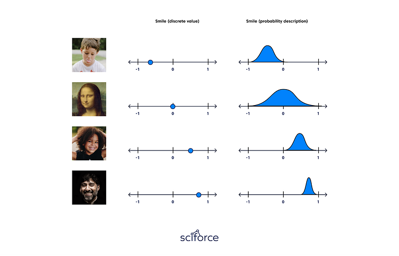
A Variational Autoencoder (VAE) is a generative model that “provides probabilistic descriptions of observations in latent spaces.” Simply put, this means VAEs store latent attributes as probability distributions.
The idea of Variational Autoencoder (Kingma & Welling, 2014), or VAE, is deeply rooted in the variational bayesian and graphical model methods.
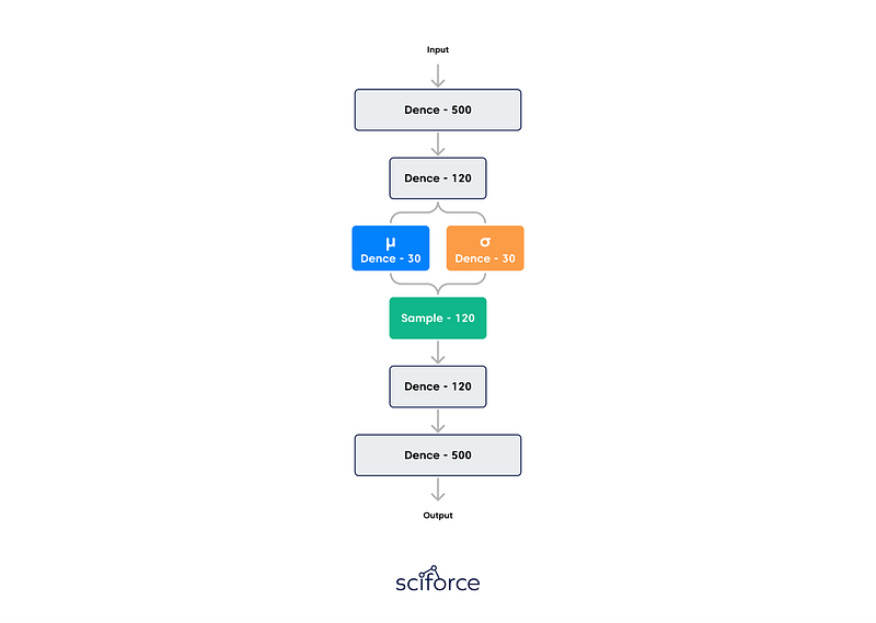
A standard autoencoder comprises a pair of two connected networks, an encoder, and a decoder. The encoder takes in an input and converts it into a smaller representation, which the decoder can use to convert it back to the original input. However, the latent space they convert their inputs to and where their encoded vectors lie may not be continuous or allow easy interpolation. For a generative model, it becomes a problem, since you want to randomly sample from the latent space or generate variations on an input image from a continuous latent space.
Variational Autoencoders have their latent spaces continuous by design, allowing easy random sampling and interpolation. To achieve this, the hidden nodes of the encoder do not output an encoding vector but_,_ rather, two vectors of the same size: a vector of means and a vector of standard deviations. Each of these hidden nodes will act as its own Gaussian distribution. The new vectors form the parameters of a so-called latent vector of random variables. The _i_th element of both mean and standard deviation vectors corresponds to the ith random variable’s mean and standard deviation values. We sample from this vector to obtain the sampled encoding that is passed to the decoder. Decoders can then sample randomly from the probability distributions for input vectors. This process is stochastic generation. It implies that even for the same input, while the mean and standard deviation remain the same, the actual encoding will somewhat vary on every pass simply due to sampling.
The loss of the autoencoder is to minimize both the reconstruction loss (how similar the autoencoder’s output to its input) and its latent loss (how close its hidden nodes were to a normal distribution). The smaller the latent loss, the less information can be encoded that boosts the reconstruction loss. As a result, the VAE is locked in a trade-off between the latent loss and the reconstruction loss. When the latent loss is small, the generated images will resemble the images at train time too much, but they will look bad. If the reconstruction loss is small, the reconstructed images at train time will look good, but novel generated images will be far from the reconstructed images. Obviously, we want both, so it’s important to find a nice equilibrium.
VAEs work with remarkably diverse types of data, sequential or nonsequential, continuous or discrete, even labeled or completely unlabelled, making them highly powerful generative tools.
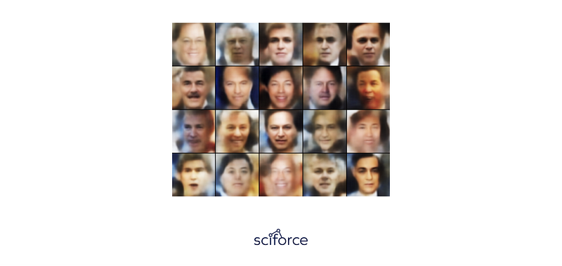
A major drawback of VAEs is the blurry outputs that they generate. As suggested by Dosovitskiy & Brox, VAE models tend to produce unrealistic, blurry samples. This is caused by the way data distributions are recovered, and loss functions are calculated. A 2017 paper by Zhao et al. has suggested modifications to VAEs not to use the variational Bayes method to improve output quality.
Generative Adversarial Networks, or GANs, are a deep-learning-based generative model that is able to generate new content. The GAN architecture was first described in the 2014 paper by Ian Goodfellow, et al. titled “Generative Adversarial Networks.”
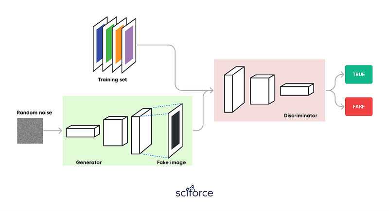
GANs adopt the supervised learning approach using two sub-models: the generator model that generates new examples and the discriminator model that tries to classify examples as real or fake (generated).
GAN sub-models
The two models compete against an adversary in a zero-sum game. The generator directly produces samples. Its adversary, the discriminator, attempts to distinguish between samples drawn from the training data and samples drawn from the generator. The game continues until the discriminator model is fooled about half the time, meaning the generator model is generating plausible examples.
Image credit: Thalles Silva
“Zero-sum” means that when the discriminator successfully identifies real and fake samples, it is rewarded, or its parameters remain the same. In contrast, the generator is penalized with updates to model parameters and vice versa. Ideally, the generator can generate perfect replicas from the input domain every time The discriminator cannot tell the difference and predicts “unsure” (e.g. 50% for real and fake) in every case. This is essentially an actor-critic model.
It is important to remember that each model can overpower the other. If the discriminator is too good, it will return values so close to 0 or 1 that the generator will struggle to read the gradient. If the generator is too good, it will exploit weaknesses in the discriminator, leading to false negatives. Both neural networks must have a similar “skill level” achieved by respective learning rates.
The generator takes a fixed-length random vector as input and generates a sample in the domain. The vector is drawn randomly from a Gaussian distribution. After training, points in this multidimensional vector space will correspond to points in the problem domain, forming a compressed representation of the data distribution. Similar to VAEs, this vector space is called a latent space, or a vector space comprised of latent variables. In the case of GANs, the generator applies meaning to points in a chosen latent space points drawn from the latent space can be provided to the generator model as input and used to generate new and different output examples.
After training, the generator model is kept and used to generate new samples.
The discriminator model takes an example as input (real from the training dataset or generated by the generator model) and predicts a binary class label of real or fake (generated). The discriminator is a normal (and well understood) classification model.
After the training process, the discriminator is discarded, since we are interested in a robust generator.
GANs can produce viable samples and have stimulated a lot of interesting research and writing. However, there are downsides to using a GAN in its plain version:
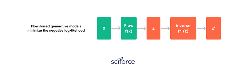
Flow-based generative models are exact log-likelihood models with tractable sampling and latent-variable inference. In general terms, Flow-Based Models apply a stack of invertible transformations to a sample from a prior so that the exact log-likelihood of observations can be computed. Unlike the previous two algorithms, the model learns the data distribution explicitly, and therefore the loss function is the negative log-likelihood.
As a rule, a flow model f is constructed as an invertible transformation that maps the high-dimensional random variable x to a standard Gaussian latent variable z=f(x), as in nonlinear independent component analysis. The key idea in the design of a flow model is that it can be any bijective function and can be formed by stacking individual simple invertible transformations. Explicitly, the flow model f is constructed by composing a series of invertible flows as f(x) =f1◦···◦fL(x), with each fi having a tractable inverse and a tractable Jacobian determinant.
Flow-based models have two large categories: models with normalizing flows and models with autoregressive flows that try to enhance the performance of the basic model.
Being able to do good density estimation is essential for many machine-learning problems. Still, it is intrinsically complex: when we need to run backward propagation in deep learning models, the embedded probability distribution needs to be simple enough to calculate the derivative efficiently. The conventional solution is to use Gaussian distribution in latent variable generative models, even though most real-world distributions are much more complicated. Normalizing Flow (NF) models, such as RealNVP or Glow, provide a robust distribution approximation. They transform a simple distribution into a complex one by applying a sequence of invertible transformation functions. Flowing through a series of transformations, we repeatedly substitute the variable for the new one according to the change of variables theorem. Then we eventually obtain a probability distribution of the final target variable.
When flow transformation in a normalizing flow is framed as an autoregressive model where every dimension in a vector variable is under the condition of the preceding dimensions, this variation of a flow model is referred to as an autoregressive flow. It takes a step forward compared to models with the normalizing flow.
The popular autoregressive flow models are PixelCNN for image generation and WaveNet for 1-D audio signals. They both consist of a stack of causal convolution — a convolution operation made considering the ordering: the prediction at a specific timestamp consumes only data observed in the past. In PixelCNN, the causal convolution is performed by a masked convolution kernel. WaveNet shifts the output by several timestamps to the future. Thus, that output is aligned with the last input element.
Flow-based models are conceptually attractive for modeling complex distributions but are limited by density estimation performance issues compared to state-of-the-art autoregressive models. Besides, though Flow Models might initially substitute GANs for producing decent output, there is a significant gap between the computational cost of training between them, with Flow-Based Models taking several times as long as GANs to generate images of the same resolution.
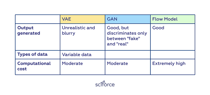
Therefore, each of the algorithms has its benefits and limitations in terms of accuracy and efficiency. While GANs and Flow-Based Models usually generate better or closer-to-life images than VAEs, the latter type is more time and parameter-efficient than Flow-Based Models.
Thus, GANs are parallel and efficient, not reversible. Flow Models, instead, are reversible and parallel but not efficient, and VAEs are reversible and efficient, but not parallel. In practice, it implies a constant trade-off between the output, the training process, and the efficiency.