
Stay informed and inspired in the world of AI with us.
 Microservices Saga – Orchestration vs Choreography
Microservices architecture has absolutely changed the approach of developers to building large and complex systems reliably. And, over the last few years, they are rapidly gaining popularity. According to the research conducted by Statista in 2021, 85% of companies utilize microservices. Well, one of the technical goals of building the application is making it scalable and secure, and microservices allow us to do this, simultaneously making the final product fault-tolerant. So, by breaking down applications into smaller, independently deployable services, microservices offer more flexibility and scalability than traditional monolithic architectures. Using this type of architecture, developers can deploy features that prevent cascading failures. Basically, there are 2 most popular approaches for implementation architecture using microservices: orchestration and choreography. And choosing the right one can be challenging. So, in this article, we would like to compare choreography and orchestration microservices architectures and discuss the projects those types of architecture are more suitable for. When it comes to microservices architecture, there are two common approaches to service coordination: orchestration and choreography. The picture above perfectly illustrates the key differences between those two approaches, and we would like to explain to you how each of them works: In this approach, a central orchestrator acts as the “brain,” or logic component, that assigns tasks to the microservices and manages and controls their interaction. In this case, the orchestrator is responsible for routing requests, coordinating service interactions, and ensuring that services are invoked in the correct order. Basically, here, the orchestrator is a central point of control and can enforce rules across the entire system. So, what are scenarios when using orchestration is more beneficial? This approach is an excellent decision when: Not suitable for large projects The first disadvantage is that the controller needs to communicate directly with each service and, after that- wait for the response of each service. The consequences here are the following: first of all, when the interactions are occurring across the network, invocations may take longer and can be impacted by downstream network and service availability. The second point is that this system can work okay in small projects, but everything can fall apart when we are talking about hundreds or even thousands of microservices. In such a case, you are creating a distributed monolithic application that will be too slow to function well. Tight coupling In the orchestration approach, microservices are highly dependent upon each other: basically, when they are synchronous, every service should respond to requests, thus, if a failure occurs - the whole process will be stopped. Moreover, if we are talking about microservices in an enterprise environment, hundreds or even thousands of microservices are attached to a single function. Therefore, this method won’t fulfill the demands of your business. Reliance on RESTful APIs Orchestration also relies on RESTful APIs, and the problem that occurs here is that RESTful APIs and orchestration can’t scale. RESTful APIs are usually created as tightly coupled services. This means that using such services increases the tight coupling of the architecture of your application. Moreover, if you would like to build new functionality, remember that it will cost a lot and have a high impact on the API. In this approach, there is no central orchestrator, and the situation is quite the opposite here: each microservice is responsible for its own behavior and coordination with other services. Services communicate with each other through events and messages without the need for a central point of control. Here, each service can react to events as they happen and can trigger events that other services can react to. To automatically apply this approach and ensure things go smoothly, you can try choreography tools like Kafka, Amazon SQS, and RabbitMQ. They all are Event Brokers, which is the main tool for this approach. A service mesh like Istio and runtime system DAPR is also used for the choreography approach. So, when should you use choreography? This approach is an excellent decision in the following cases: Avoiding the creation of a single point of failure or bottleneck is important for you. You need microservices to be autonomic and independent. You want to simplify the process of adding or removing services from the system without disrupting the overall flow of communication. Now, let’s discuss the benefits of choreography that are solving the problems that occur with orchestration: Loose service coupling for agility and fault tolerance Well, adding and removing services is much simpler using a choreographed microservices architecture. Basically, here you will only need to connect/disconnect the microservice to the appropriate channel in the event broker. So, using loose service coupling, the existing logic will not fall apart when you add or remove microservices. And this results in less development churn and flux. Moreover, because of the independence of each service, when one application fails, the whole system will work while the issue is rectified as choreography isolates microservices. Also, it is not required to have a built-in error handling system in case of failure of the network, as this responsibility lies on the event broker. Faster, more agile development As clients' requirements are higher every day and the market grows constantly, the speed of development and modifying the app is crucial. So, the development teams are impacted by changes to other services, and it is a common barrier to achieving agility. But, here, choreographed microservices enable development teams to focus on their key services and operate more independently. So, the services are easily shared between teams once they are created. This allows us to save labor, time, and resources. More consistent, efficient applications During the creation of microservices with specific functions, you can create a more modular codebase. In this case, each microservice by itself has its business function, and together, microservices perform a business process. Thus, your system will be consistent, and it will be easy to modify and create services because you can reuse your microservices and tap into code that’s already been proven to perform a given function. So, what are the different and similar features between microservices and orchestration? Let us briefly summarise this: Both approaches involve service coordination and communication and can be used to implement complex workflows and business processes and build scalable and maintainable microservices architectures. When deciding between orchestration and choreography, it's important to consider the specific needs of your project. Here are some of the most important factors to consider:
 Serving ML model as an API- Sharing our experience
Serving machine learning models as an API is a common approach for integrating ML capabilities into modern software applications. This process helps to simplify the development of applications and has multiple benefits, such as scalability, efficiency, flexibility, and accessibility. Basically, the aim of such an API is to integrate machine learning models into other components of the application, which enables the use of the predictive power of machine learning in real time. So, this process allows systems to use the model's predictions and insights without having to replicate the entire architecture and infrastructure of the model. And today, we would like to share with you our experience in serving the ML model as an API. In this article, we'll walk you through this process and cover the following aspects and steps: Features: Pros: Cons: Features: Pros: Cons: Features: Pros: Cons: Features: Pros: Cons: Choose a deployment platform: You can choose to deploy your API to a server or a cloud-based platform such as Amazon Web Services, Google Cloud Platform, or Microsoft Azure. Consider factors such as scalability, cost, and ease of use when choosing a deployment platform. Set up the environment: Once you've chosen a deployment platform, set up the environment by installing any required dependencies and configuring the server or cloud-based platform. Upload your API code: Upload your API code to the server or cloud-based platform. This can be done by copying the code files to the server or by using a version control system such as Git to push the code to a repository. Configure the API endpoint: Configure the API endpoint on the server or cloud-based platform. This involves specifying the URL for the API endpoint, any required parameters, and any security settings such as authentication and authorization. Test the deployed API: After deploying the API, test it to ensure that it works as expected. You can use the same testing tools, such as Postman that you used during the development phase. Monitor and maintain the API: Once the API is deployed, monitor it to ensure that it is performing well and that it is meeting the required service level agreements (SLAs). You may need to update and maintain the API over time as new features are added or as the underlying technology changes. By deploying your API, you make it accessible to users and allow it to be used in production environments. This can provide significant benefits such as increased efficiency, scalability, and accessibility. Monitoring the API is an important step that will help you ensure that the whole system performs well and meets your requirements. Here are some of the key things you should monitor:
 Top Microservices Design Patterns for Your business
Using microservices for building apps is rapidly gaining popularity as they can bring so many different benefits to the business: they are safe and reliable, scalable, optimize the development time and cost, and are simple to deploy. In our previous articles, we discussed the best tools to manage microservices, the advantages and disadvantages of using microservices and the differences they have with monolith architecture, and hexagonal architecture. Despite multiple benefits, app development with microservices has many challenges: Advantages: Disadvantages: When to use the Strangler pattern When not to use Advantages: Disadvantages: When to use the Saga pattern When not to use Saga Advantages: Disadvantages: When to use the Aggregator Pattern When not to use the Aggregator Pattern Advantages: Disadvantages: When to use Event Sourcing When not to use Event Sourcing Advantages: Disadvantages: When to use CQRS When not to use CQRS Disadvantages: When to use Backends for Frontends When not to use Backends for Frontends
 Top Java Trends in 2021
Well, 2020 has proved that making predictions is at least naive today. But when it comes to the mid or long-term investment decisions, things are getting more serious. It is also crucial for developers to plan their careers and invest time efficiently. So please welcome the most significant trends of Java that will help you stay tuned up. Java remains among the most popular languages for web, desktop, and mobile development and embedded software. It was the only official language for Android development until 2017 when Kotlin entered the picture. Simultaneously, it is not that easy to find out what share of apps on the Google Store uses Java. For instance, hybrid applications like React Native, Cordova, PhoneGap, and Iconic have Java under the hood having the business logic of JS. Also, it is not easy to refer to the robust statistics, but eight of the eleven most traffic-generating websites worldwide are using Java, at least for the back-end programming. That fact gives us a clear vision of its strength and popularity. Moreover, Tomcat and Elasticsearch, among the most popular web servers and search engines for enterprises, are also using Java. Meanwhile, despite being one of the favorite choices and time-tested, Java is also adopting megatrends like cloud deployment and containerization. We are delving into it step-by-step. The trend of cloud computing emerged even before the Covid-19 pandemic, but now things are accelerating. On average, every person uses 36 cloud-based servicess every day, and 81% of all enterprises are working on their multi-cloud strategy. Per Gartner, spending on public cloud services will grow from $270 billion in 2020 to $332.3 billion this year, which is more than 23% higher. But how Java space has already reacted to it, and what comes next? You probably have noticed the increased adoption of AWS and some other cloud services due to the rise of containerized workloads. Thus, cloud-native and Kubernetes-supporting frameworks like Micronaut, Quarks, and Spring Boot become even more popular. Spring Boot, the leader of this domain, eliminates boilerplate configurations required to set up Spring applications. It has features like an embedded server opinionated “starter” dependencies that lead to the simplified building and configuring of the applications. Health checks, metrics, and externalized configurations come as a pleasant bonus. Micronaut is reported to be the first platform in Java that is efficiently working in a serverless architecture. It can’t compete with Spring Boot in popularity but holds about 5k stars on GH as per writing. Though Micronaut has some features resembling the Spring, it boasts of the compile-time dependency injection mechanism. This framework builds its dependency injection data at compile-time, differing from the majority of frameworks. As a result, you can enjoy smaller memory footprints and faster application startup. Moreover, Micronaut also boasts great support for reactive programming for clients and servers. Both RxJava and Project Reactor are supported. It also supports multiple service discovery tools like Eureka and Consul, and different distributed tracing systems like Zipkin and Jaeger. Quarkus released by Red Hat in 2019, is holding about 8k stars on GH as of the moment of writing. Erik Costlow, Java Editor at InfoQ, pointed out that Quarkus is using the best parts of the cloud, Jakarta EE, and GraalVM. It automates container creation and has a rapid reload. Moreover, Quarkus uses its plugin ecosystem that connects to the other systems. When needed, you also can turn for detailed documentation for each plugin. It supports Kubernetes, Hibernate, OpenShift, Kafka, and Vert.x. With Quarkus, developers can concentrate on code instead of technical work and interaction with resources. Moreover, it is built on top of the standards, so you should not learn anything new. GraalVM and static compilation are the crucial building blocks of the going cloud. GraalVM boasts of features like ahead-of-time compilation (AOT), uses features and libraries of the most popular languages, and provides debugging, monitoring, profiling, and resource consumption optimization tools. Spring, Quarkus, Micronaut, and Helidon frameworks are integrated with GraalVM. Java 8 and 11 are still the most usable updates at the moment. As per the JetBrains 2020 survey, 75% of the respondents are opting for Java 8, leaving another update in second place. The newest update on the SE platform, as of the moment, JDK 16, was in March 2021, making it the latest Java trend. It boasts 17 enhancements like JVM improvements, new tools, libraries category, incubator, and preview feature to improve your productivity. The SE 15 includes improvements like: Records to declare a class since it is added automatically: toStrings, hashCode, getters, equals methods, and constructor. Hidden classes, usually dynamically generated at runtime, can’t be accessible by the name, and you can not link them to the other classes’ byte code. Also, JDK 17 is likely to enter the picture in September 2021, so stay tuned. Since Oracle does not provide Java binaries at zero cost longer than six months after release, the market is opting for non-Oracle providers like AdoptOpenJDK, Azul, and Amazon. Java also follows megatrends like cloud computing and serverless architecture, so cloud-native supporting frameworks are gaining momentum. Micronaut, Quarks, and Spring Boot are among them, letting developers concentrate on the code instead of infrastructure. Java 8 LTS is still the most popular, but JDK 17 is likely to enter the picture in September 2021. Meanwhile, there is no trend to beat Java 8 so far. Got inspired? Do not forget to clap for this post and give us some inspiration back!
 Containerization, Docker, Docker Compose: Step-by-step Guide
Before we delve into the details of Docker and Docker Compose, let us define the principal idea of containerization. Skip to the following blocks without any ado if you are eager to reveal Docker’s nuts and bolts immediately. To the rest of the readers:” Welcome on board, cabin boys and girls!” Container technology today is mainly associated with Docker, which also helped to accelerate the overall trend of native cloud development. Meanwhile, technology is rooted in the 1970s, as Rani Osnat tells in his blog on container’s brief history. Containerization, in essence, packages up code with all its dependencies that it can run on any infrastructure. It is often accompanied by virtualization or stands as an alternative. Usually, a team of developers working on some applications has to install all the needed services on their machines directly. For instance, for some JS applications, you would need PostgreSQL v9.3 and Redis v5.0 for messaging. That also means that every developer in your team or testers should also have these services installed. The installation process differs per OS environment, and there are many steps where something could go wrong. Moreover, the overall process could be even trickier depending on the application’s complexity. To better grasp the idea, let’s describe the typical workflow before using containers. Development teams produce artifacts with some instructions. You’d have a jar file or something like this with the list of instructions on how to configure and a database file with the same list of instructions for server configuration. The development team would give these files to the operations team, and they would set up the environment to deploy those applications. In this case, the operations team would have everything installed on their OS that could lead to dependency version conflicts. Moreover, some misunderstandings between the teams may also arise since all the instructions are in textual format. For example, developers could miss some crucial points regarding configuration, or the operations team could misinterpret something. Consequently, this could lead to some sort of back and forth communication between the teams. With containers, these processes are actually simplified. Now the development and operations team could be on the same page using the containers. No environmental configuration is needed on the server, except Docker Runtime. You need to run the docker command to pull the application image from the repository to run it. No environmental configuration is required on the server as you have set up the Docker Runtime on the server. That is just a one-time effort. So, you need not look for packages, libraries, and other software components for your machine and start working using this container. All you need is to download a specific repository on your local machine. One command is the same regardless of the OS you are using. For example, if you need to build some JS application, you need to download and install only the containers required for this application, and that is it. There are two different technical terms — Docker image and Docker container. Images are the actual packages (Configuration + PostgreSQL v9.3+ Start script), i.e., it is an artifact that is movable around this image. The container is layers of stacked images on top of each other. Most of the containers are mostly Linux Base images because of being lightweight. On top of the base image, you would have an application image. When you download an image and install it on your machine, it starts the application and creates a container environment. It is not running in the Docker image, and the container is the exact thing running on your machine. Docker — is a containerization platform that packages applications into containers, combining source code with all the dependencies and libraries of the operating system. With containers, it is possible to run code in any environment. Docker, in essence, provides the toolkit for developers to build, deploy, and run containers using basic commands and automation. Thus, it is easy to manage containers using Docker. Docker Inc. provides an enterprise edition (Docker EE) and an open-source project. What is the difference between container and image? The container is a running environment for the image. For example, application images (PostgreSQL, Redis, Mongo DB) that may need a file system, log files, or any environmental configurations — all of this environmental stuff provided by the container. The container also contains a port that allows talking to an application running inside the container. What is Docker Hub? Docker Hub contains images only. Every image on Docker Hub has different versions (you can select the latest version by default when you have no dependencies). Check out also the list of the basic Docker commands. People often use the terms “Docker” and “container” interchangeably nowadays, so it is hard to define some cons, but we tried to provide a well-balanced list. Let’s start with benefits: Efficient usage of resources Docker containers make not only the apps isolated from each other but the OS. This way, you can dictate how to use system resources like GPU, CPU, and memory. It also helps to make a cleaner software stack and keep code and data separately. Compared to virtual machines (VMs), containers are very lightweight and flexible. Since every single process could run in a single container, you could easily update or repair containers when needed. Moreover, when there is a need to optimize Docker images for the best performance with less effort, it is also possible. Check out how we have optimized the size of Docker images by over 50% in blog _Strategies of docker images optimization__._ Improved portability You can use Docker and do not take care of machine-specific configuration since applications are not tied to the host OS. This way, both the application and host environment are clean and minimal. Of course, containers are built per specific platforms (container for Windows won’t launch on macOS and vice versa), but there is a solution for this case. It is called manifest and is still in its experimental phase. In essence, it is images for multiple OSs packed in one image, so that Docker could be both a cross-environmental and cross-platform solution. Enhanced microservices model In general, software consists of multiple components grouped into a stack, like a database, in-memory cache, and web-server. With containers, you can manage these pieces as one functional unit with changeable parts. Each part is based on a different container, so you can easily update, change or modify any of them. Check out our ever-green blog _Microservices: how to stay smart and avoid trendy words_ for more details. Since containers are lightweight and portable, you can quickly build and maintain microservice-based architecture. You can even reuse existing containers as a base of images (i.e., templates) to make new containers. Orchestration and scaling Since containers are lightweight and use resources efficiently, it is possible to launch lots of them. You can also tailor them for your needs and amount of resources, using third-party projects like Kubernetes. In essence, it provides automatic orchestration and scaling of the containers, like a scheduler. Docker also provides its system, Swarm mode. Meanwhile, Kubernetes is a leader by default. Both solutions (Docker and Kubernetes) are bundled with Docker Enterprise Edition. However, Docker is not a silver bullet for all your needs. Thus, consider the following: Docker is not a VM Docker and VMs are using different virtualization mechanisms since the first one virtualizes only the application layer. VM virtualizes the complete OS — both the applications layer and the OS kernel. VM has its Guest OS, while Docker is running on the Host OS. Thus, Docker is smaller and faster than VM. But, Docker is not that compatible as VM that you can run on any host OS. Before installing Docker, check whether your OS can host Docker natively. If your OS can not run Docker, you need to install Docker Toolbox to create a bridge between your OS and Docker that enables it to run on your computer. Docker containers do not have persistency and immutability Docker’s image is immutable by default. That means that when you have created it, you can not change it. The same is about the persistency — you won’t have any stateful information when restarting the container associated with the old one. It also differs from VMs with persistency through the sessions by default since it has a file system. Thus, containers’ statelessness makes developers keep the application’s data and code separately. The installation differs not only per OS but the version of the specific OS. Thus, we strongly recommend checking the prerequisites before installation. For Mac and Windows, some OS and hardware criteria have to be met to support running Docker. For example, it runs only on Windows 10 natively. For Linux process is different per distribution. As we have mentioned, if your OS can not run Docker, you need to install Docker Toolbox that creates a bridge between your OS and Docker that enables it to run on your computer. By installing Docker, you will have the whole package — Docker Engine, a necessary tool to run the Docker containers on your laptop. Docker CLI client will enable you to execute some Docker commands, and Docker Compose is a technology that helps you orchestrate multiple containers, and we are covering it further. For Mac users, it is crucial to know that once you have multiple accounts on your laptop, you could experience errors if you will run Docker on various accounts. Do not forget to quit Docker on the account when switching to another one when you use Docker on that account top. Windows users should have virtualization enabled while installing Docker on Windows. Virtualization is by default always enabled if you have not disabled it manually. Download the Docker file and follow the Wizard guides to run Docker. You need to start Docker manually after installation since it won’t start automatically. Docker Compose, in essence, is a superstructure above Docker. You can easily use Docker Engine for a few containers, but it is impossible with lots of them. So, Docker Compose (which is also automatically installed within the complete package) comes in handy. It is an orchestration and scheduling tool to manage the application’s architecture. Docker Compose uses YAML file specifying the services included in the application and can run and deploy the applications using one command. With Docker Compose, you can define a constant volume for storage, configure service dependencies, and specify base nodes. You did it! A journey of a thousand miles begins with a single step, and here is your first one. Docker will help to develop software simply and efficiently. And with Docker Compose, you will orchestrate containers. Moreover, a robust community stands behind this technology to not be alone in your journey of mastering the best DevOps practices.
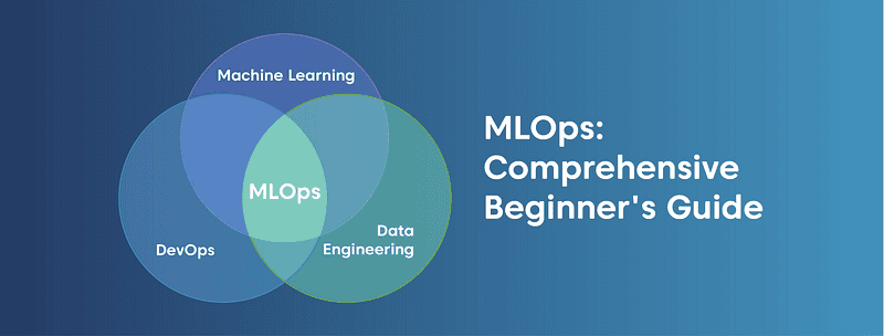 MLOps: Comprehensive Beginner’s Guide
MLOps, AIOps, DataOps, ModelOps, and even DLOps. Are these buzzwords hitting your newsfeed? Yes or no, it is high time to get tuned for the latest updates in AI-powered business practices. Machine Learning Model Operationalization Management (MLOps) is a way to eliminate pain in the neck during the development process and delivering ML-powered software easier, not to mention the relieving of every team member’s life. Let’s check if we are still on the same page while using principal terms. Disclaimer: DLOps is not about IT Operations for deep learning; while people continue googling this abbreviation, it has nothing to do with MLOps at all. Next, AIOps, the term coined by Gartner in 2017, refers to the application cognitive computing of AI & ML for optimizing IT Operations. Finally, DataOps and ModelOps stand for managing datasets and models and are part of the overall MLOps triple infinity chain Data-Model-Code. While MLOps seems to be the ML plus DevOps principle at first glance, it still has its peculiarities to digest. We prepared this blog to provide you with a detailed overview of the MLOps practices and developed a list of the actionable steps to implement them in any team. Per Forbes, the MLOps solutions market is about to reach $4 billion by 2025. Not surprisingly that data-driven insights are changing the landscape of every market’s verticals. Farming and agriculture stand as an illustration with AI’s value of 2,629 million in the US agricultural market projected for 2025, which is almost three times bigger than it was in 2020. To illustrate the point, here are two critical rationales of ML’s success — it is the power to solve the perceptive and multi-parameters problems. ML models can practically provide a plethora of functionality, namely recommendation, classification, prediction, content generation, question answering, automation, fraud and anomaly detection, information extraction, and annotation. MLOps is about managing all of these tasks. However, it also has its limitations, which we recommend to bear in mind while dealing with ML models production:
 The Strength and Beauty of GraphQL in Use
Facebook developed GraphQL as a major problem-solver for more efficient mobile data loading in 2012 and released it as an open-source solution three years later. Since that time, it mistakenly associates with PHP only and lacks trust given Facebook’s reputation (if you know what I mean). However, a recent Netflix case that finds GraphQL as a game-changer to power the API layer and increase the scalability and operability of the studio ecosystem attracts attention. This specification already gained popularity — given State of JavaScript 2019 Report, 50.6% of respondents have heard of GraphQL and would like to learn it. However, The New York Times, Airbnb, Atlassian, Coursera, NBC, GitHub, Shopify, and Starbucks are already among the GraphQL users. We decided to dwell on the beauty, strength, and some constructions of GraphQL in its scalability, performance, and security aspects and tell about our use cases for a banking sphere and a platform of commercial targeting. See the list of useful toolkits added at the end as a bonus. GraphQL is a convenient way of communication between a client and a server. Sometimes one can see it as an opponent to REST API given the main difference that GraphQL brings to the table — the only endpoint to fetch the data by one call from multiple sources. Meanwhile, we are to provide the space for consideration of whether this specification is relevant to particular tasks or whether REST API is the silver bullet for your case. Both REST and GraphQL APIs are stateless, supported by any server-side language and any frontend framework, and exchange the data through the JSON. But the one and only endpoint containing the query expression to define the data that should be returned creates the what-you-see-is-what-you-get principle to optimize the work. Let’s deep dive into the specification’s main advantages and disadvantages. The flexibility of GraphQL is its main advantage over REST, as one gets what they want in a single API request. Define the structure of the information to receive back, and it goes back in the format requested, no under-fetching or over-fetching. Meanwhile, caching seems to be one of the GraphQL downsides compared to REST (see the complete list of all the pros and cons further). REST APIs use the HTTP caching mechanism, providing cached data faster. It leverages its community-powered and time-tested feature, leaving GraphQL behind at the moment. Security is another area of improvement for GraphQL when comparing it with REST, which boasts a more mature system. The latter leverages HTTP authentication, JSON Web Tokens (JWT), or OAUth 2.0 mechanisms. Unlike REST API, GraphQL has detailed documentation and supports the function of nested queries that contributes to the principle “no over fetching and under fetching data,” which happened while using the first specification. Query and mutation are the joint GraphQL operations. Thus, the CRUD (create, read, update, delete) model is not relevant for GraphQL as the create operation executes through the query command (other ones are implemented with mutations). Advantages Disadvantages The Platform for Commercial Targeting GraphQL became a convenient solution for one of our clients who needed to develop a platform for commercial targeting, providing a straightforward approach for searching the potential customers in any national institution or facility. Using it, the client can direct the ads straight to the audience of interest using geolocation data and a set of filters. The platform consists of two primary services: one for geo-based consumer extraction based on PlaceIQ dataset usage and one for attribute-based (consumers identity graph) with consumer dataset. The project can be extended by adding the missing residential dataset to retrieve residents at the requested addresses. Also, the services could be wrapped into the REST API to provide the ability to trigger them using web requests. Risk Reduction and Resilience Boosting Financial Platform An average bank encounters no more than 100K transactions a day. Moreover, it also faces malicious actions and the risk of cyberattacks. One of our clients needed to empower their software platform to encounter higher transaction pressure and provide a higher risk-management system to avoid financial crimes. As a result, we have developed a solution that stands for the high amount of transactions and provides reports while detecting anomalies based on the transactions’ data in real-time. Check out the growing GraphQL community to find the latest updates on this solution. There are many horizontally and vertically developed solutions for GraphQL client, GraphQL gateway, GraphQL server, and database-to-GraphQL servers. Add some of the tools that you enjoy using while working with GraphQL in the comments to this blog. GraphQL’s servers are available for languages like JavaScript, Java, Python, Perl, Ruby, C#, Go, etc. Apollo Server for JavaScript applications and GraphQL Ruby are some of the most popular choices. Apollo Client, DataLoader, GraphQL Request, and Relay are among popular GraphQL clients. Graphiql, GraphQL IDE, and GraphQL Playground for IDE’s respectively. Some handy tools:
 Strategies of docker images optimization
Docker, an enterprise container platform is developers’ favorite due to its flexibility and ease of use. It makes it generally easy to create, deploy, and run applications inside of containers. With containers, you can gather applications and their core necessities and dependencies into a single package turn it into a Docker image, and replicate it. Docker images are built from Dockerfiles, where you define what the image should look like, as well as the operating system and commands. However, large Docker images lengthen the time it takes to build and share images between clusters and cloud providers. When creating applications, it’s therefore worth optimizing Docker Images and Dockerfiles to help teams share smaller images, improve performance, and debug problems. A lot of verified images available on Docker Hub are already optimized, so it is always a good idea to use ready-made images wherever possible. If you still need to create an image of your own, you should consider several ways of optimizing it for production. As a part of a larger project, we were asked to propose ways to optimize Docker images for improving performance. There are several strategies to decrease the size of Docker images to optimize for production. In this research project, we tried to explore different possibilities that would yield the best boost of performance with less effort. By optimization of Docker images, we mean two general strategies: 9667e45447f6 About an hour ago /bin/sh -c apt-get update 27.1MB a2a15febcdf3 3 weeks ago /bin/sh -c #(nop) CMD \[“/bin/bash”\] 0B <missing> 3 weeks ago /bin/sh -c mkdir -p /run/systemd && echo ‘do… 7B <missing> 3 weeks ago /bin/sh -c set -xe && echo ‘#!/bin/sh’ > /… 745B <missing> 3 weeks ago /bin/sh -c [ -z “$(apt-get indextargets)” ] 987kB <missing> 3 weeks ago /bin/sh -c #(nop) ADD file:c477cb0e95c56b51e… 63.2MB ``` When it comes to measuring the timings of Dockerfile steps, the most expensive steps are COPY/ADD and RUN. The duration of COPY and ADD commands cannot be reviewed(unless you are going to manually start and stop timers), but it corresponds to the layer size, so just check the layer size using `docker history` and try to optimize it. As for RUN, it is possible to slightly modify a command inside to include a call to \`time\` command, which would output how long it take `RUN time apt-get update` But it requires many changes in Dockerfile and looks poorly, especially for commands combined with && Fortunately, there’s a way to do that with a simple external tool called gnomon. Install NodeJS with NPM and do the following sudo npm i -g gnomon docker build | gnomon The output will show you how long either step took: … 0.0001s Step 34/52 : FROM node:10.16.3-jessie as node\_build 0.0000s — -> 6d56aa91a3db 0.1997s Step 35/52 : WORKDIR /tmp/ 0.1999s — -> Running in 4ed6107e5f41 … One of the most interesting pieces of information you can gather is how your build process performs when you run it for the first time and when you run it several times in a row with minimal changes to source code or with no changes at all. In an ideal world, consequent builds should be blazingly fast and use as many cached layers as possible. In case when no changes were introduced it’s better to avoid running a docker build. This can be achieved by external build tools with support for up-to-date checks, like Gradle. And in case of small minor changes, it would be great to have additional volumes be proportionally small. It’s not always possible or it might require too much effort, so you should decide how important is it for you, which changes you expect to happen often and what’s going to stay unchanged, what is the overhead for each build, and whether this overhead is acceptable. And now let’s think of the ways to reduce build time and storage overheads. It is always wise to choose a lightweight alternative for an image. In many cases, they can be found on existing platforms: FROM ubuntu:14.04 # 188 MB FROM ubuntu:18.04 # 64.2MB There are even more lightweight alternatives for Ubuntu, for example Alpine Linux: FROM alpine:3 # 5.58MB However, you need to check if you depend on Ubuntu-specific packages or libc implementation (Alpine Linux uses musl* instead of *glibc). See the comparison table. Another useful strategy to reduce the size of the image is to add cleanup commands to apt-get install commands. For example, the commands below clean temporary apt files left after the package installation: ``` RUN apt-get install -y && \ unzip \ wget && \ rm -rf /var/lib/apt/lists/* && \ apt-get purge --auto-remove && \ apt-get clean ``` If your toolkit does not provide tools for cleaning up, you can use the rm command to manually remove obsolete files. RUN wget www.some.file.xz && unzip www.some.file.xz && rm www.some.file.xz Cleanup commands need to appear in the RUN instruction that creates temporary files/garbage. Each RUN command creates a new layer in the filesystem, so subsequent cleanups do not affect previous layers. It is well-known that static builds usually reduce time and space, so it is useful to look for a static build for C libraries you rely on. Static build: ``` RUN wget -q https://johnvansickle.com/ffmpeg/builds/ffmpeg-git-amd64-static.tar.xz && \ tar xf ffmpeg-git-amd64-static.tar.xz && \ mv ./ffmpeg-git-20190902-amd64-static/ffmpeg /usr/bin/ffmpeg && \ rm -rfd ./ffmpeg-git-20190902-amd64-static && \ rm -f ./ffmpeg-git-amd64-static.tar.xz # 74.9MB ``` Dynamic build: `RUN apt-get install -y ffmpeg # 270MB` The system usually comes up with recommended settings and dependencies that can be tempting to accept. However, many dependencies are redundant, making the image unnecessarily heavy. It is a good practice to use the `--no-install-recommends` flag for the apt-get install command to avoid installing “recommended” but unnecessary dependencies. If you do need some of the recommended dependencies, it’s always possible to install them by hand. RUN apt-get install -y python3-dev # 144MB RUN apt-get install --no-install-recommends -y python3-dev # 138MB As a rule, a cache directory speeds up installation by caching some commonly used files. However, with Docker images, we usually install all requirements once, which makes the cache directory redundant. To avoid creating the cache directory, you can use the `--no-cache-dir` flag for the pip install command, reducing the size of the resulting image. RUN pip3 install flask # 4.55MB RUN pip3 install --no-cache-dir flask # 3.84MB A multi-stage build is a new feature requiring Docker 17.05 or higher. With multi-stage builds, you can use multiple FROM statements in your Dockerfile. Each FROM instruction can use a different base, and each begins a new stage of the build. You can selectively copy artifacts from one stage to another, leaving behind everything you don’t want in the final image. ``` FROM ubuntu:18.04 AS builder RUN apt-get update RUN apt-get install -y wget unzip RUN wget -q https://johnvansickle.com/ffmpeg/builds/ffmpeg-git-amd64-static.tar.xz && \ tar xf ffmpeg-git-amd64-static.tar.xz && \ mv ./ffmpeg-git-20190902-amd64-static/ffmpeg /usr/bin/ffmpeg && \ rm -rfd ./ffmpeg-git-20190902-amd64-static && \ rm -f ./ffmpeg-git-amd64-static.tar.xz FROM ubuntu:18.04 COPY --from=builder /usr/bin/ffmpeg /usr/bin/ffmpeg # The builder image itself will not affect the final image size # the final image size will be increased only to /usr/bin/ffmpeg file’s size ``` Although builder stage image size will not affect the final image size, it still will consume disk space of your build agent machine. The most straightforward way is to call `docker image prune` But this will also remove all other dangling images, which might be needed for some purposes. So here’s a more safe approach to removing intermediate images: add a label to all the intermediate images and then prune only images with that label. ``` FROM ubuntu:18.04 AS builder LABEL my_project_builder=true docker image prune --filter label=my_project_builder=true ``` Multi-stage builds are powerful instruments, but the final stage always implies COPY commands from intermediate stages to the final image and those file sets can be quite big. In case you have a huge project, you might want to avoid creating a full-sized layer, and instead take the previous image and append only a few files that have changed. Unfortunately, COPY command always creates a layer of the same size as the copied fileset, no matter if all files match. Thus, the way to implement incremental layers would be to introduce one more intermediate stage based on a previous image. To make a diff layer, rsync can be used. ``` FROM my_project:latest AS diff_stage LABEL my_project_builder=true RUN cp /opt/my_project /opt/my_project_base COPY --from=builder /opt/my_project /opt/my_project RUN patch.sh /opt/my_project /opt/my_project_base /opt/my_project_diff FROM my_project:latest LABEL my_project_builder=true RUN cp /opt/my_project /opt/my_project_base COPY --from=builder /opt/my_project /opt/my_project RUN patch.sh /opt/my_project /opt/my_project_base /opt/my_project_diff ``` Where patch.sh is the following ``` #!/bin/bash rm -rf $3 mkdir -p $3 pushd $1 IFS=’ ‘ for file in \`rsync -rn --out-format=”%f” ./ $2\`; do [ -d “$file” ] || cp --parents -t $3 “$file” done popd ``` For the first time, you will have to initialize my\_project:latest image, by tagging the base image with the corresponding target tag `docker tag ubuntu:18.04 my_project:latest` And do this every time you want to reset layers and start incrementing from scratch. This is important if you are not going to store old builds forever, cause hundreds of patches might consume more than ten full images. Also, in the code above we implied rsync is included in the builder’s base image to avoid spending extra time for installing it on every build. The next section is going to present several more ways to save the build time. The most obvious solution to reduce build time is to extract common packets and commands from several projects into a common base image. For example, we can use the same image for all projects based on the Ubuntu/Python3 and dependent on unzip and wget packages. A common base image: FROM ubuntu:18.04 RUN apt-get update && \\ apt-get install python3-pip python3-dev python3-setuptools unzip wget A specific image: FROM your-docker-base RUN wget www.some.file CMD \[“python3”, “your\_app.py”\] To prevent copying unnecessary files from the host, you can use a .dockerignore file that contains all temporarily created local files/directories like .git, .idea, local virtualenvs, etc.. Docker uses caching for filesystem layers, where in most cases each line in the Dockerfile produces a new layer. As there are layers that are more likely to be changed than others, it is useful to reorder all commands according to the probability of changes in the ascending order. This technique saves you time by rebuilding only the layers that have been changed so that you can copy source files when you need them. Unordered command sequence: FROM ubuntu:18.04 RUN apt-get update COPY your\_source\_files /opt/project/your\_source\_files RUN apt-get install -y `--`no-install-recommends python3 Ordered command sequence: FROM ubuntu:18.04 RUN apt-get update RUN apt-get install -y `--`no-install-recommends python3 COPY your\_source\_files /opt/project/your\_source\_files Sometimes, one of the most time-consuming steps for big projects is dependencies downloading. It is inevitable to perform at least once, but consequent builds should use cache. Surely, layer caching could help in this case — just separate dependencies downloading step and actual build: COPY project/package.json ./package.json RUN npm i COPY project/ ./ RUN npm run build However, the resolution will happen once you increment any minor version. So if slow resolution is a problem for you, here’s one more approach. Most dependencies resolution systems like NPM, PIP, and Maven support local cache to speed up consequent resolution. In the previous section, we wrote how to avoid leaking of pip cache to the final image. But together with incremental layers approach it is possible to save it inside an intermediate image. Setup an image with rsync, add a label like `` `stage=deps` `` and prevent that intermediate image from being removed by cleanup `docker images --filter label=my\_project\_builder=true --filter label=stage=deps --filter dangling=true --format {{.ID}} | xargs -i docker tag \{\} my\_project/deps` Then let the builder stage depend on my\_project/deps image, perform build, and copy compiled files to the final image. Such intelligent implementation of optimization strategies allowed us to reduce the Docker image size by over 50% giving significant increase in the speed of image building and sharing. Feel free to share your best practices of writing better Dockerfiles in the comments below.
 Data Cleaning and Preprocessing for Beginners
When our team’s project scored first in the text subtask of this year’s CALL Shared Task challenge, one of the key components of our success was careful preparation and cleaning of data. Data cleaning and preparation is the most critical first step in any AI project. As evidence shows, most data scientists spend most of their time — up to 70% — on cleaning data. In this blog post, we’ll guide you through these initial steps of data cleaning and preprocessing in Python, starting from importing the most popular libraries to actual encoding of features. Data cleansing* or **data cleaning** is the process of detecting and correcting (or removing) corrupt or inaccurate records from a record set, table, or database and refers to identifying incomplete, incorrect, inaccurate or irrelevant parts of the data and then replacing, modifying, or deleting the dirty or coarse data. //*Wikipedia The absolutely first thing you need to do is to import libraries for data preprocessing. There are lots of libraries available, but the most popular and important Python libraries for working on data are Numpy, Matplotlib, and Pandas. Numpy* is the library used for all mathematical things. **Pandas** is the best tool available for importing and managing datasets. *Matplotlib (Matplotlib.pyplot) is the library to make charts. To make it easier for future use, you can import these libraries with a shortcut alias: _import numpy as np import matplotlib.pyplot as plt import pandas as pd_ Once you downloaded your data set and named it as a .csv file, you need to load it into a pandas DataFrame to explore it and perform some basic cleaning tasks removing information you don’t need that will make data processing slower. Usually, such tasks include: _You should also pay attention to data leakage_, which can cause the model to overfit. This is because the model will be also learning from features that won’t be available when we’re using it to make predictions. We need to be sure our model is trained using only the data it would have at the point of a loan application. With a filtered data set explored, you need to create a matrix of dependent variables and a vector of independent variables. At first you should decide on the appropriate column to use as a target column for modelling based on the question you want to answer. For example, if you want to predict the development of cancer, or the chance the credit will be approved, you need to find a column with the status of the disease or loan granting ad use it as the target column. For example, if the target column is the last one, you can create the matrix of dependent variables by typing: _X = dataset.iloc\[:, :-1\].values_ That first colon (:*) means that we want to take all the lines in our dataset. **: -1** means that we want to take all of the columns of data except the last one. The `.*values` on the end means that we want all of the values. To have a vector of independent variables with only the data from the last column, you can type _y = dataset.iloc\[:, -1\].values_ Finally, it’s time to do the preparatory work to feed the features for ML algorithms. To clean the data set, you need to handle missing values and categorical features*, because the mathematics underlying most machine learning models assumes that the data is numerical and contains no missing values. Moreover, the *scikit-learn library returns an error if you try to train a model like linear regression and logistic regression using data that contain missing or non-numeric values. Missing data is perhaps the most common trait of unclean data. These values usually take the form of NaN or None. here are several causes of missing values: sometimes values are missing because they do not exist, or because of improper collection of data or poor data entry. For example, if someone is under age, and the question applies to people over 18, then the question will contain a missing value. In such cases, it would be wrong to fill in a value for that question. There are several ways to fill up missing values:
 Our Adaptation of Lyon’s Auditory Model for Python
In contrast to our usual theoretical posts, in this story, we will discuss our recent adaptation of the popular Lyon’s auditory model for Python. The ability of the human auditory system to recognize speech in adverse and noisy conditions has prompted researchers to introduce features of human perception in speech recognition systems. The early 1980s saw an outburst of computational models based on physiological measurements of the response of individual auditory nerve fibers. One of the models that emerged at that time was Lyon’s passive longwave cochlear model. The original Lyon’s auditory model is a part of the auditory toolbox written for MATLAB. This toolbox is useful for researchers and speech and auditory engineers who want to see how the human auditory system represents sounds. Richard F. Lyon, an American scientist and prominent inventor, described an auditory model showing the propagation of sound in the inner ear and the conversion of acoustical energy into neural representations followed by several stages of adaptation. The model simulates the behavior of the cochlea, the most important part of the inner ear. In its essence, the cochlea is a non-linear filter bank: thanks to the variability of its stiffness, different places along it are sensible to sounds with different spectral content. However, the model does not try to literally describe each structure in the cochlea but treats it as a “black box.” Like the sound entering the cochlea is converted into nerve firings that travel up the auditory nerve into the brain, the model outputs a vector proportional to the firing rate of neurons at each point in the cochlea. The cochlear model combines a series of filters that recreate the traveling pressure waves with Half Wave Rectifiers (HWR) to detect the energy in the signal and several stages of Automatic Gain Control (AGC): This behavior is simulated by a cascade filter bank. The number of such filters depends on the sampling rate of the signals, the overlapping factor of the filter band, the quality of the resonant part of the filters, and other factors. The more filters the more accurate is the model. The model results in maps of auditory nerve firing rates, called cochleagrams. Cochleagrams are a variation of spectrograms and refer to two-dimensional time-frequency representations that are used to better reveal spectral information. While at a coarse temporal scale, cochleagrams and spectrograms look quite similar except for the scale of the frequency axis, cochleagrams can preserve more of the fine time scale structure of each sound component, e.g. the glottal pulses. Written for C and MATLAB, the computer adaptation for Lyon’s passive longwave cochlear model implements multiple stages of the multiplicative adaptive gain. Its input is a number of channels from a filter bank. An array of state filters, one per channel and per stage, measure a running average of the energy in the channel. These variables are then used to drive a single multiplicative gain per stage per channel. In our speech recognition project, we experimented with waveform segmentation and ASR, and it turned out that Lyon’s model-based features outperformed standard MFE and MFCC features. However, we used Python for the project, and we could not find any previous implementation of Lyon’s model for Python, only the original C code from AuditoryToolbox. Moreover, from the global perspective, increasingly more AI-related projects are written in Python, so we found it useful to port Lyon’s model to this language. To successfully call `LyonPassiveEar()` we removed the MEX-related part from `soscascade.c`, `agc.c` and `sosfilters.c`, made a `ctypes` wrapper for `soscascade()`, `agc()` and `sosfilters()` calls and translated the necessary files from MATLAB to Python. A complete description and the installation guide for the project can be found on the corresponding PyPI page. If you want to test how it works, you can use our code to compute a cochleogram for a sample sound: from* lyon *import LyonCalc calc = LyonCalc() waveform, sample\_rate = load('audio/file/path.wav') decimation\_factor = 64 coch = calc.lyon\_passive\_ear(waveform, sample\_rate, decimation\_factor) print(coch.shape) The code above outputs the shape of the resulting auditory nerve response: `[<number of samples / decimation_factor>, 86]`. We hope that adapting this famous model for Python will be a helpful addition to Python’s range of NLP tools and will help further work on speech processing. Richard F. Lyon (b. 1952) is an influential American inventor and engineer. One of the key figures in signal processing, he worked on both optical and auditory signals. He is the author of a cochlear model that is used as the basis of much auditory research and optical and integrated-circuit techniques. For instance, this model improved the accuracy of digital color photography. Lyon was one of two people who independently invented the first optical mouse device. He also designed early Global Positioning System test transmitters and the first single-chip Ethernet device. In 2017, Lyon published his first book, _Human and Machine Hearing: Extracting Meaning from Sound_.
